Wish I Knew How to Sort (an exercise in probability)

In this post I would like to talk about solving Codeforces 1753C: Wish I Knew How to Sort.

In the exercise we receive a binary array $a$ with $n$ elements, which we want to sort. However, our algorithms teacher forgot to teach us about sorting algorithms. :)

For lack of a better idea, we choose a randomized method, in which a step looks like the following:

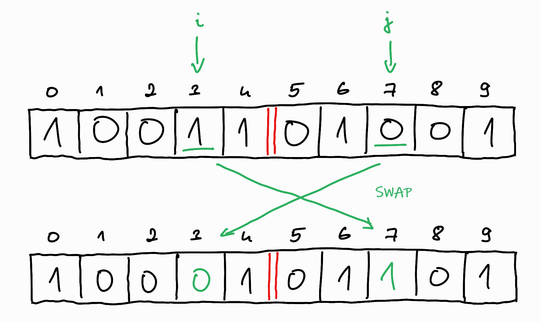
• We point to two positions in the array at random (with uniform distribution, independently of each other and of our previous steps). Let these be denoted by indices $i$ and $j$, where $i < j$.
• If they are in the wrong order ($a_i > a_j$), we swap them, otherwise we do nothing.

This step is repeated until the array is sorted.

Question: What is the expectation value of the steps taken?

In the task, there is a technical detail that the solution must be written as an irreducible fraction (a fraction that can no longer be simplified), I will cover the method of doing this at the end.

There are at least two very different solutions to the task, both of which are very useful to know for handling probabilistic exercises.

Observation

The first thing we can observe is that we know how many $0$s and $1$s are in the $a$ array, so we can already draw the borer between the $0$s and the $1$s in the resulting, sorted array.

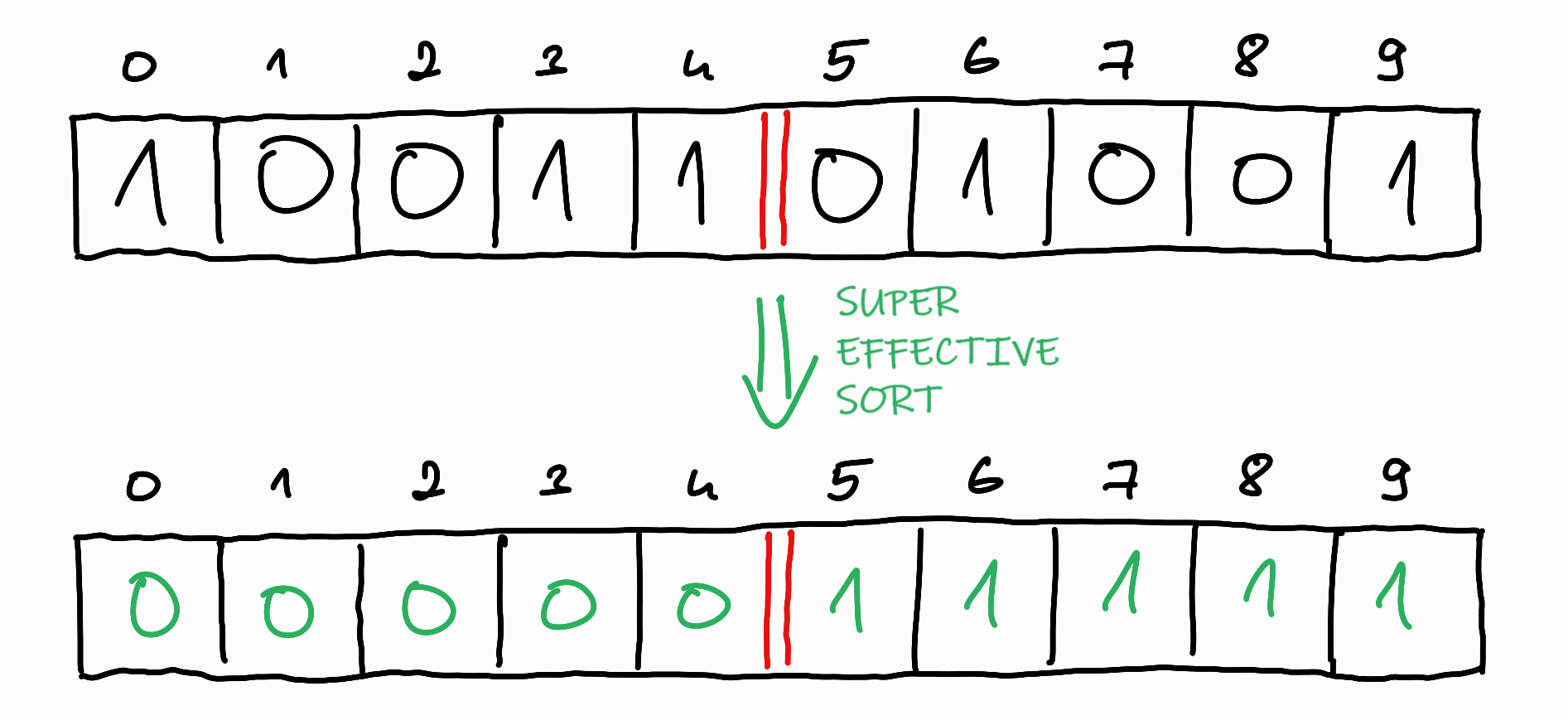
Then, based on the location of the randomly chosen pair $i < j$, there are actually two different cases:

1. $i$ is before the dividing line, $j$ is after it.
2. Both are before or after the dividing line.

In the first case, if there is a swap, we have done useful work, since we have increased the number of $0$s before the line and the number of $1$s after the line, bringing us closer to the desired state.

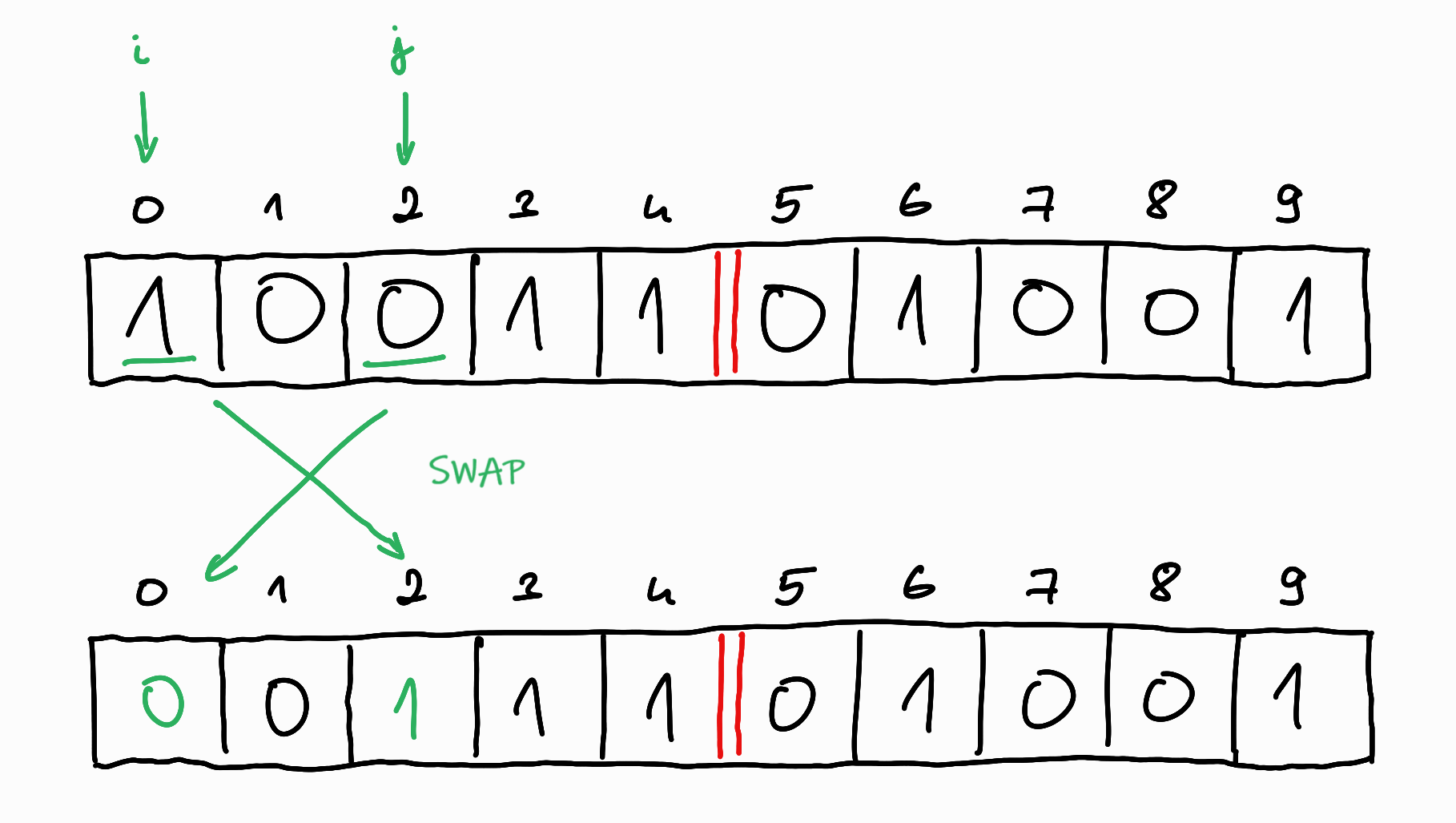
In the second case, if there is a swap, we did not do useful work with it, since we only moved things within the border, we still have to move the same amount of $1$s from the left side of the border to the right side and replace them with $0$s.

So it can be said that the exact location of the $0$s and $1$s is irrelevant, the only thing that matters is how many of them are on either side of the boundary line. A useful step occurs only when $i$ is before the boundary and $j$ is after the boundary, and $a_i = 1$ and $a_j = 0$. In all other cases, the step does not change the current state.

First method: Geometric distribution and linearity of the expectation value

If you know probability theory, you may recognize a notable distribution in the task: this is the geometric distribution. This appears when we “repeat something until something occurs”.

A little detour: about the geometric distribution (for those who don’t know it yet)

More precisely:

1. We perform a series of random experiments.
2. Among the possible outcomes of the experiments, we distinguish between “successful” and “failed” outcomes.
   • We call a set of outcomes an event, so we have a “successful” and a “failed” event.
   • The probability of the “successful” event is known, let’s denote it by $p$, the probability of the “failed” event is therefore $1-p$.
3. The individual experiments are performed independently of each other (i.e. the probability of success is not affected by the results of the previous experiments).
4. We stop when we get a successful result.
5. We define a random variable that tells us how many steps we took before we stopped.

For example, if the variable $X$ represents the number of steps, we can ask what the probability is that exactly $i$ steps were taken, i.e. $P(X=i) = ?$.

This requires $i-1$ failed attempts and $1$ successful attempt, so

\(P(X=i) = (1-p)^{i-1}p\).

And the possible values of $i$ are any number of steps between $1$ and $\infty$.

The advantage of knowing notable distributions is, for example, that we know their expectation value. We denote this for the variable $X$ by $E(X)$. By definition, the expectation value is the sum of the possible values of a variable weighted by their probability, i.e

\[E(X) = \sum\limits_{i} i \cdot{} P(X=i).\]

(We can later talk about the fact that if we sample $X$ many times, i.e. carry out the series of random experiments and write down how many steps we took, then the average of the obtained step numbers will get closer and closer to this theoretical expectation value, but now we are in the territory of statistics. )

The expectation value of the geometric distribution

The theoretical expectation value of the geometric distribution is $\frac{1}{p}$, which can be easily calculated by substituting into the formula above:

\[E(X) = \sum\limits_{i} i \cdot{} P(X=i) = \sum\limits_{i} i \cdot{} (1-p)^{i-1}p = p \sum\limits_{i=1}^{\infty} i \cdot{} (1-p)^{i-1}\]

We have come across such infinite sums many times and they can be dealt with in many ways. Now we are mainly bothered by the $i$ multiplier, without which we would have a geometric series, so we should get rid of it.

For example, we start from the original equality and see what it looks like if we start to expand it:

\[E(X) = p \sum\limits_{i=1}^{\infty} i \cdot{} (1-p)^{i-1} = p + 2p(1-p) + 3p(1-p)^2 + 4p(1-p)^3 + \cdots{}\]

Multiply both sides by $(1-p)$:

\[(1-p) E(X) = p \sum\limits_{i=1}^{\infty} i \cdot{} (1-p)^{i} = p(1-p) + 2p(1-p)^2 + 3p(1-p)^3 + 4p(1-p)^4 + \cdots{}\]

We notice that if we subtract the two from each other, we can get rid of the $i$ multipliers and get the sum of an infinite geometric series:

\[E(X) - (1-p) E(X) = p + p(1-p) + p(1-p)^2 + p(1-p)^3 + p(1-p)^4 + \cdots{} = p \sum\limits_{i=0}^{\infty} (1-p)^{i} = p \cdot{} \frac{1}{1-(1-p)} = 1\]

So

\[E(X) - E(X) + pE(X) = 1,\] \[pE(X) = 1,\] \[E(X) = \frac{1}{p}.\]

It is worth remembering this result.

Back to the task

There is some kind of “do it until we succeed” feeling about the task, so we believe there is some geometric random variable in the background, the expectation value of which we now know. Let’s try to model the task in this way!

It is quickly seen that a single variable is not enough to model the problem. Let’s think about it: then the stopping condition would be that the array has become sorted, for which a fixed probability $p$ would have to be determined, which should also be the same in each step, since the steps are independent. It won’t work that way. The steps are not independent this way.

Instead, we can distribute the steps among several random variables: let the successful event be the one when our randomly chosen indices $i$ and $j$ fall on different sides of the boundary line and a swap is performed. There will be more than one of this event, which means we will need more than one random variables. However, fortunately, we can already tell from the initial array $a$ exactly how many variables are needed: as many successful events as are needed, i.e. how many $1$s are on the left side of the boundary: let’s denote this number with $k$ !

Then the number of steps needed can be described as the sum of $k$ variables. Let $X_i$ be the variable that describes the number of steps needed to move from $i$ to $i-1$ number of $1$s on the left side (so that the last step was the only successful and useful swap in the sequence of steps needed).

Then the number of steps can be described by the sum of the variables $X_k + X_{k-1} + \cdots{} + X_1$, we need to calculate the expectation value of this sum, i.e. $E(X_k + X_{k-1} + \cdots{} + X_1)$.

Here we use a very important theorem, the linearity of expectation, i.e

\[E(X_k + X_{k-1} + \cdots{} + X_1) = E(X_k) + E(X_{k-1}) + \cdots{} + E(X_1).\]

What is very surprising in this formula is that it is true even if the individual variables are not independent of each other and there are competitive programming tasks that strongly depend on this property. This is not the case now, here our variables will be independent, so this is perhaps less surprising, but for those of you, more interested in the topic, you can read about it here, for example: https://brilliant.org/wiki/linearity-of-expectation/.

Then we only need to give a formula for $E(X_i)$. If there $i$ number of $1$s on the left side, then the probability of a successful swap, $p_i$ can be given with the formula favourable / total number of cases as follows:

• Since the array has $n$ elements, the total number of cases is how many ways I can choose an ordered pair of indices from the elements, this is $\binom{n}{2}$.
• The number of favourable cases is how many ways I can choose a $1$ on the left side of the boundary and a $0$ on the right side.
• If there are $i$ pieces of $1$s on the left side, it means that there are the same number of $0$s on the right side, and we want to choose a pair of them, so $i\cdot{}i = i^2$ is the number of favourable cases.

So

\[p_i = \frac{i^2}{\binom{n}{2}}.\]

And it follows that the expectation value of a variable

\[E(X_i) = \frac{1}{p_i} = \frac{\binom{n}{2}}{i^2}.\]

And the expectation value of the sum is

\[E = E(X_k) + E(X_{k-1}) + \cdots{} + E(X_1) = \sum\limits_{i=1}^{k}\frac{\binom{n}{2}}{i^2}.\]

At this point, we have solved the problem on a theoretical level, the only thing left to do is calculating this sum programatically.

Before we do that, let’s first look at a completely different solution:

Second method: Markov chain hitting times with dynamic programming

A little detour: about Markov chains (for those who don’t know it yet)

In probability theory, Markov chains describe random processes that fulfill some kind of memorylessness criteria. Now I’m just going to talk about a special type of these, but for simplicity I’m just going to refer to them as Markov chains.

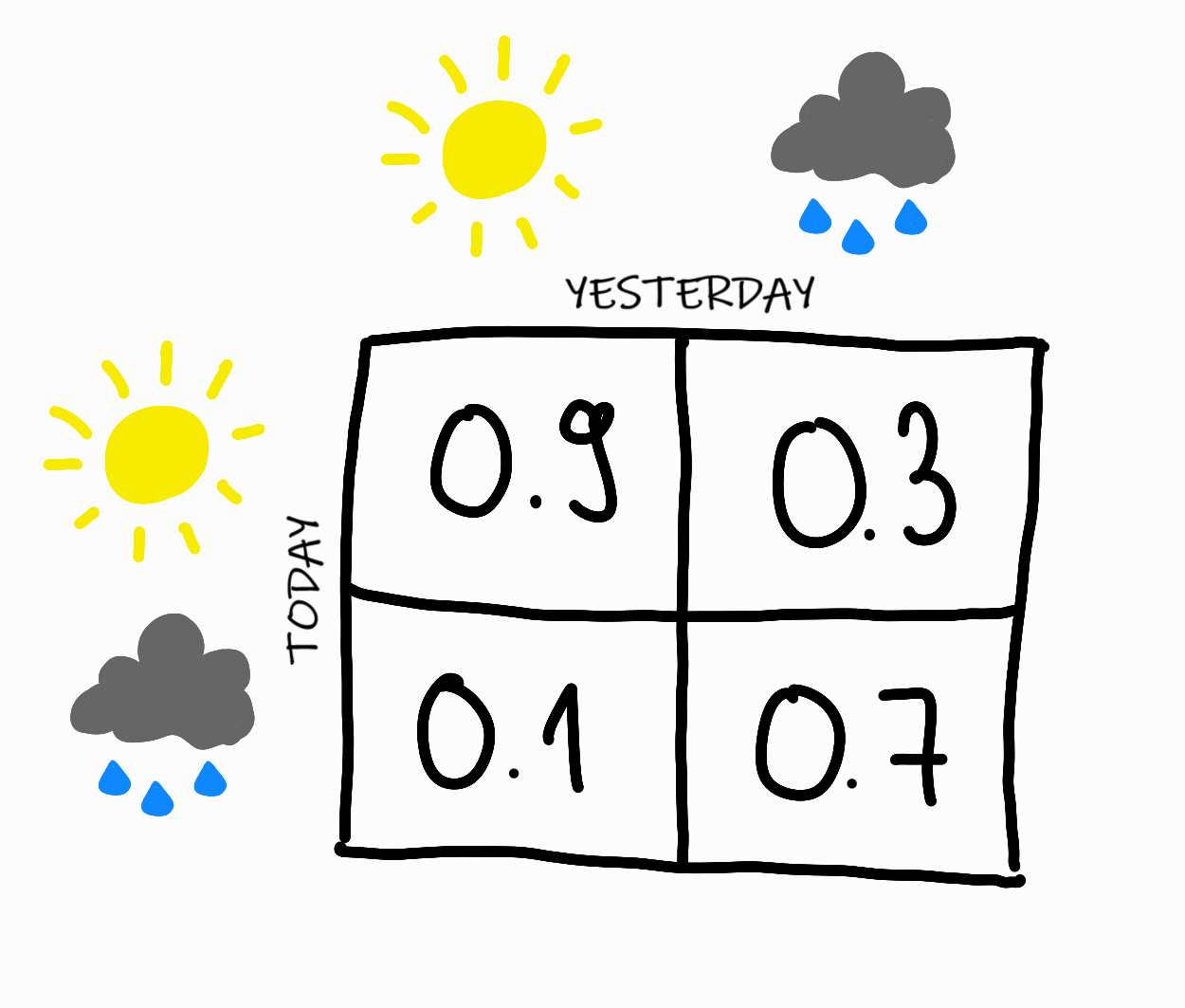
For example, imagine a weather model that says:

• If the sun was shining yesterday, there is a $90\%$ probability that the sun will also be shining today.
• If it rained yesterday, there is a $70\%$ probability that it will also rain today.

These statements can be illustrated with a diagram:

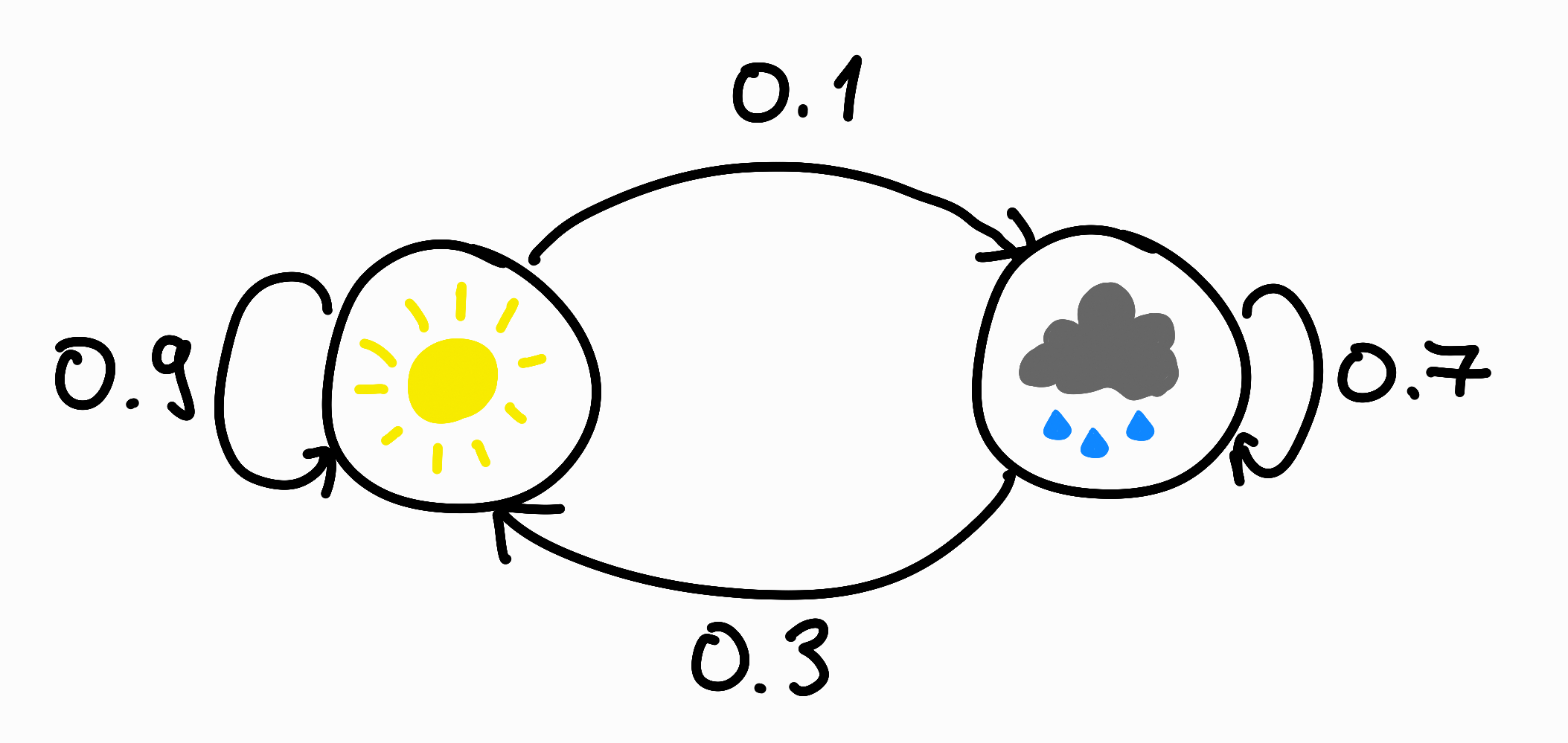
This is an example of a very simple Markov chain. The chain has $2$ possible states, “sunny” and “rainy”. The random variable $X_i$ indicates the weather on day $i$. The above statements can be translated into the language of probability, with which we can specify the state transition probabilities of the chain:

• The probability that the weather is sunny on day $i$, provided that it was also sunny on the previous day, $i-1$: $P(X_i = sunny \vert X_{i-1} = sunny) = 0.9$
• The probability that the weather is rainy on day $i$, provided that it was sunny on the previous day, $i-1$: $P(X_i = rainy \vert X_{i-1} = sunny) = 0.1$
• The probability that the weather is sunny on day $i$, provided that it was rainy on the previous day, $i-1$: $P(X_i = sunny \vert X_{i-1} = rainy) = 0.3$
• The probability that the weather is rainy on day $i$, provided that it was also rainy on the previous day, $i-1$: $P(X_i = rainy \vert X_{i-1} = rainy) = 0.7$

This can be described in a concise way by the transition probability matrix (usually denoted by $\Pi$):

The matrix is stochastic, meaning that the sum of any column is $1$, since it is partition of the sample space:

• The events are pairwise disjoint, since according to our model there can only be one type of weather on a day.
• Their union is the entire sample space, since according to our model there is some kind of weather every day.

The memorylessness condition (or the so-called Markov condition) here means that the weather of a given day depends only on the weather of the previous day, “not on the weather of any other past days”. This latter description worded mathematically correctly goes: if yesterday’s weather is known, today’s weather is independent of the weather of all other previous days.

Back to the task

In our exercise, we can recognize a similar Markov chain. The states of this should correspond to the number of $1$s on the left side of the boundary. We know that the possible values are $0, \dots{}, k$, where $k$ is the value belonging to the starting array.

We have previously specified the $p_i$ probabilities, which will be the transitional probabilities of this chain:

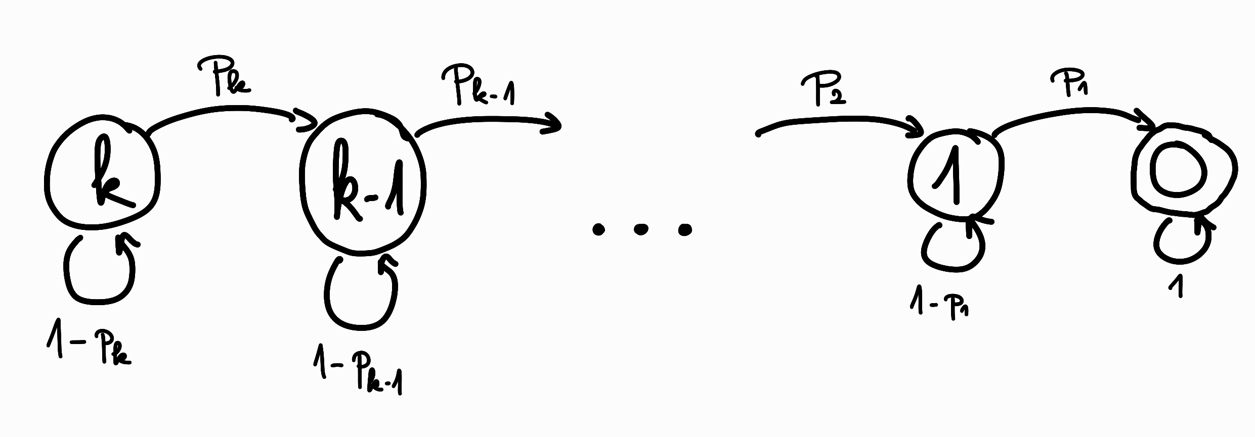
Now the question is, what is the expectation number of steps until the chain reaches from state $k$ to state $0$?

This is the so-called “hitting time” of the chain.

It can be derived in general [1], as follows: [1]: https://mpaldridge.github.io/math2750/S08-hitting-times.html

Let’s denote by $\nu_{j\leftarrow{}i} = \nu_{j,i}$ that if the current state of the Markov chain is $i$, then what is the expectation value of the number of steps before it first reaches state $j$.

• If $i = j$, then $\nu_{i,i} = 0$.
• In any other case, at least one step is required to reach state $j$.
  • This one step will enter another state $s$, according to the probabilities written on the outgoing edges of state $i$.
  • This other state $s$ also has some hitting time towards the target state.
  • Due to the linearity of expectation, the following “self-referential formula” can be given:
    • $S$ denotes the set of possible states.
    • $p_{s,i}$ denotes value written in the transition probability matrix in row $s$ and column $i$, i.e. the probability of moving from state $i$ to state $s$.

\[\nu_{j,i} = 1 + \sum\limits_{s\in{}S} \nu_{j,s}p_{s,i}\]

Here we used the Law of total expectation.

This results in a very nice dynamic programming solution for our Markov chain.

• Since we want to reach state $0$, the only question is which state we came from, denote this with $k$.
• Let $dp[k]$ denote the hitting time from state $k$ to $0$.
• We know that in the case of $k\neq{}0$, at least one step must be taken.
• This step can be unsuccessful (with probability $1-p_k$) or successful (with probability $p_k$).
• Substitute this into the general formula above:

\[dp[k] = 1 + (1-p_k) dp[k] + p_k dp[k-1]\]

• And rearrange:

\[p_k \cdot{} dp[k] = 1 + p_k \cdot{} dp[k-1]\] \[dp[k] = \frac{1}{p_k} + dp[k-1]\]

• Furthermore:

\[dp[0] = 0\]

This clearly shows that

\[dp[k] = \sum\limits_{i=1}^{k} \frac{1}{p_k}\]

Which is exactly the same formula that we derived from the geometric distribution solution! :)

Printing the solution as an irreducible fraction

In the case of the first method, the following sum must be calculated:

\[E = \sum\limits_{i=1}^{k}\frac{\binom{n}{2}}{i^2} = \frac{n(n-1)}{2}\sum\limits_{i=1}^{k}\frac{1}{i^2}\]

Let’s bring the fractions in the sum to a common denominator!

Let $D$ be the common denominator!

\[D = \prod\limits_{i=1}^{k}i^2\] \[E = \frac{n(n-1)}{2} \frac{\sum\limits_{i=1}^{k}\frac{D}{i^2}}{D} = \frac{P}{Q}\]

This is good for us, because the numerator and denominator of this fraction must be integer, so we can calculate them separately:

\[P = n(n-1) \sum\limits_{i=1}^{k}\frac{D}{i^2}\] \[Q = 2D\]

And in Python, the third parameter of the pow function is the modulo, so the inverse of $Q$ with the modulo can be determined with it to calculate $\frac{P}{Q}$.

Source code:

cases = int(input())
   
for _ in range(cases):
     
  n = int(input())
  a = list(map(int, input().split()))
     
  border = 0 # Where is the border between the 0s and 1s of the final result.
  for i in range(n):
    if a[i] == 0:
      border += 1
        
  k = 0 # The number of 1's before the border, that need to be swapped to the other side.
  for i in range(border):
    if a[i] == 1:
      k += 1

  if k==0:
    print(0)
    continue

  D = 1
  for i in range(1, k+1):
    D *= i*i

  S = 0
  for i in range(1, k+1):
    S += D / (i * i)
  P = n*(n-1) * S

  Q = 2 * D

  mod = 998244353
  QInv = pow(Q, -1, mod)
  
  print(int((P * QInv) % mod))

And this results in a time limit exceeded at the moment. :) (TODO)